A Gentle Introduction to Linear Algebra

Introduction

The purpose of today's post is to gather the essential linear algebra prerequisites that support deep learning. It is meant as a summary. Our topic is the fundamental building blocks of linear algebra: scalars, vectors, and matrices.

Scalar & Vector

A scalar $k \in \mathbb{R}$ is a quantity that can be represented by a real number but has no direction. A vector, on the other hand, is a geometric object that has both a numerical magnitude and a direction. The conventional notation $\mathbf{v} = \begin{bmatrix} x_1 \\ ... \\ x_n \end{bmatrix}$, $x_1, ..., x_n \in \mathbb{R}$ is in the form of a column matrix. The number of rows of a vector indicates the dimension of the space it belongs to, such that $\mathbf{v} \in \mathbb{R}^n$ is an element of the n-dimensional real space.

Vector Addition and Scalar Multiplication

Matching components are added. Note that vectors of different dimensions cannot be added.

$$\mathbf{u} + \mathbf{v} = \begin{bmatrix} u_{x_1} \\ u_{x_2} \end{bmatrix} + \begin{bmatrix} v_{x_1} \\ v_{x_2} \end{bmatrix} = \begin{bmatrix} u_{x_1} + v_{x_1} \\ u_{x_2} + v_{x_2} \end{bmatrix} \quad \mathbf{u},\mathbf{v} \in \mathbb{R}^{2}$$

Multiplying a vector by a scalar means multiplying each component by that scalar.

$$k \cdot \mathbf{v} = k \cdot \begin{bmatrix} v_x \\ v_y \end{bmatrix} = \begin{bmatrix} k \, v_x \\ k \, v_y \end{bmatrix} \quad k \in \mathbb{R}, \quad \mathbf{v} \in \mathbb{R}^{2}$$

Vector Length (Norm)

The length (Euclidean norm) of a vector is the square root of the sum of the squares of its components:

$\|\mathbf{v}\| = \sqrt{x_1^2 + x_2^2 + \cdots + x_n^2}$

Unit Vector

Vectors with a length of 1 unit, that is, satisfying the condition $\|\mathbf{v}\| = 1$, are called unit vectors. They are used to represent coordinate axes.

$\mathbf{v} = \begin{bmatrix} x_1 \\ x_2 \end{bmatrix} = x_1\begin{bmatrix} 1 \\ 0 \end{bmatrix} + x_2\begin{bmatrix} 0 \\ 1 \end{bmatrix}$

The equation above is an example of a linear combination of a vector with unit vectors in two-dimensional space.

Geometric Interpretation of Vectors

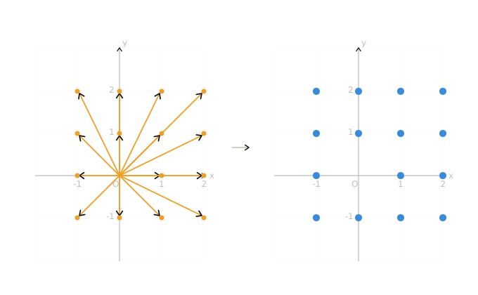
$x_1, ..., x_n$ are called coordinate axes. Each coordinate axis measures the length of the vector along that axis. The origin $O=(0, ... , 0) \in \mathbb{R}^n$ is the starting point for all vectors. Therefore, every point in space represents a vector whose starting point is the origin.

Figure 1: An example of vector and point correspondence in two-dimensional space.

Matrix

Unfortunately, no one can be told what the Matrix is. You have to see it for yourself.

— Morpheus

A matrix is the numerical representation of a linear transformation that keeps the origin fixed, preserves lines as lines, and does not break the parallelism of parallel lines. Formally, for a transformation $T$ to be linear, it must satisfy the following two conditions:

$T(\mathbf{u}+\mathbf{v}) = T(\mathbf{u}) + T(\mathbf{v}), \newline T(k\mathbf{v}) = kT(\mathbf{v})$

This definition covers operations such as rotation, reflection, scaling, shearing, and projection.

Let $A \in \mathbb{R}^{m \times n}$. Then $A$ is a matrix of size $m \times n$, where $m$ is the number of rows and $n$ is the number of columns.

$$A = \begin{bmatrix} a_{11} & a_{12} & \cdots & a_{1n} \\ a_{21} & a_{22} & \cdots & a_{2n} \\ \vdots & \vdots & \ddots & \vdots \\ a_{m1} & a_{m2} & \cdots & a_{mn} \end{bmatrix}$$

Matrix Addition and Multiplication

$A = \begin{bmatrix} a_{11} & a_{12} \\ a_{21} & a_{22} \end{bmatrix} \quad \text{and} \quad B = \begin{bmatrix} b_{11} & b_{12} \\ b_{21} & b_{22} \end{bmatrix}$ be two matrices. The addition and multiplication operations are as follows.

$$A + B = \begin{bmatrix} a_{11} & a_{12} \\ a_{21} & a_{22} \end{bmatrix} + \begin{bmatrix} b_{11} & b_{12} \\ b_{21} & b_{22} \end{bmatrix} = \begin{bmatrix} a_{11}+b_{11} & a_{12}+b_{12}\\ a_{21}+b_{21} & a_{22}+b_{22} \end{bmatrix}$$ $$AB = \begin{bmatrix} a_{11} & a_{12} \\ a_{21} & a_{22} \end{bmatrix} \begin{bmatrix} b_{11} & b_{12} \\ b_{21} & b_{22} \end{bmatrix} = \begin{bmatrix} a_{11}b_{11} + a_{12}b_{21} & a_{11}b_{12} + a_{12}b_{22} \\ a_{21}b_{11} + a_{22}b_{21} & a_{21}b_{12} + a_{22}b_{22} \end{bmatrix}$$

The intuition behind defining matrix multiplication this way is as follows: matrix multiplication is the composition of transformations. The expression $AB$ means applying transformation $B$ first and then transformation $A$. This intuition is the key to understanding why successive layers in deep learning are expressed through matrix multiplication. Matrix multiplication is not commutative: in general, $AB \neq BA$. Changing the order of transformations yields a different result.

Transpose of a Matrix

$\text{For an } m \times n \text{ matrix } A \text{, its transpose } A^{\top} \text{ is an } n \times m \text{ matrix:}$

$A = \begin{bmatrix} a_{11} & a_{12} & a_{13} \\ a_{21} & a_{22} & a_{23} \end{bmatrix} \quad \Longrightarrow \quad A^{\top} = \begin{bmatrix} a_{11} & a_{21} \\ a_{12} & a_{22} \\ a_{13} & a_{23} \end{bmatrix}$

The general rule is $(A^{\top})_{ij} = A_{ji}$.

Symmetric Matrix

A square matrix whose transpose equals itself is called a symmetric matrix.

$A = A^{\top} \quad \Longleftrightarrow \quad a_{ij} = a_{ji} \quad \forall\, i, j$

In deep learning, symmetric matrices such as the covariance matrix, Hessian, and Gram matrix are frequently encountered.

Geometric Interpretation of Matrix & Vector

Multiplying a matrix by a vector applies the linear transformation represented by that matrix to the vector.

$$\begin{bmatrix} a & b \\ c & d \end{bmatrix} \begin{bmatrix} x \\ y \end{bmatrix} = x\begin{bmatrix} a \\ c \end{bmatrix} + y\begin{bmatrix} b \\ d \end{bmatrix} = \begin{bmatrix} ax+by \\ cx+dy \end{bmatrix}$$

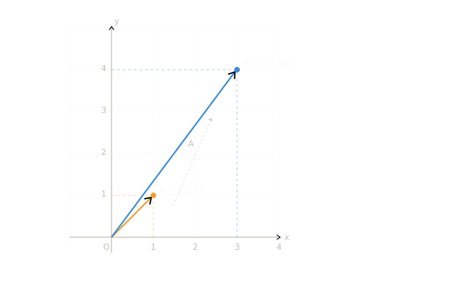
Let's work through an example: $\newline A = \begin{bmatrix} 2 & 1 \\ 1 & 3 \end{bmatrix} \in \mathbb{R}^{2 \times 2}$ be a matrix and $\mathbf{v} = \begin{bmatrix} 1 \\ 1 \end{bmatrix} \in \mathbb{R}^{2}$ be a vector.

$$\mathbf{v'} = A\mathbf{v} = \begin{bmatrix} 2 & 1 \\ 1 & 3 \end{bmatrix} \begin{bmatrix} 1 \\ 1 \end{bmatrix} = \begin{bmatrix} 2\cdot1 + 1\cdot1 \\ 1\cdot1 + 3\cdot1 \end{bmatrix} = \begin{bmatrix} 3 \\ 4 \end{bmatrix}$$

The new vector resulting from the matrix multiplication $\mathbf{v'} = \begin{bmatrix} 3 \\ 4 \end{bmatrix}$ is the linear transformation of $\mathbf{v}$. That is, the vector has been transformed — its direction and magnitude have changed.

Figure 2: The orange vector represents $\mathbf{v}$, and the blue vector represents $\mathbf{v'}$.

Conclusion

Linear algebra is one of the best tools we have for modeling the spaces we scientifically explore. Fitting all those spaces onto paper is no small feat. If the reader wishes to dive deeper, they can explore the resources below.

See you in the next post!

References

1. Dive into Deep Learning
2. Essence of Linear Algebra — 3Blue1Brown